I finally find the time to deliver on a promise I made on tweeter: to talk about genome assembly.
A few months ago, a discussion on a tweeter thread was opened on the art of assembling genomes. Of course, I will not be addressing which is the best assembly program or the best parameter to obtain the best N50, it is completely dependent on the sample's nature and sequencing process. Instead, we are going to get a hold of an arsenal of tools to get to the soul of a genome, get to know its most unresolved contigs, its most repeated repetitions, its most hidden extrachromosomal elements and, incidentally, some assembly errors.
First off, let me introduce you to a program that begins its history in the 90s. It is known as the 'Staden Package' and its publication begins with the following abstract…
Methods Mol Biol. 2000;132:115-30. doi: 10.1385/1-59259-192-2:115. [PUBMEDID]
The Staden Package, 1998
R Staden 1 , K F Beal, J K Bonfield
I [the author] describe the current version of the sequence analysis package developed at the MRC Laboratory of Molecular Biology, which has come to be known as the «Staden Package.» The package covers most of the standard sequence analysis tasks such as restriction site searching, translation, pattern searching, comparison, gene finding, and secondary structure prediction, and provides powerful tools for DNA sequence determination. Currently the programs are only available for computers running the UNIX operating system. Detailed information about the package is available from our WWW site: http:@www.mrc-lmb.cam.ac.uk/pubseq/.
The main website can be found at: http://staden.sourceforge.net/
ATTENTION: In order to follow this explanation / tutorial, prior knowledge of genome assembling and mapping is required.
Let's begin this journey with a primary assembly with a few contigs in mind. It can be an assembly obtained with any of the plethora of assembly programs for first, second, and third generation sequencing data, or a hybrid assembly built from several technologies. The purpose of the Staden package is to evaluate and check any contig obtained in the primary assembly in order to break, merge, annotate, etc. the assemblies' contigs.
First of all, we define «contig» as a fragment of a contiguous sequence.
We start from contigs of an Escherichia coli genome assembly obtained with any assembler with any parameters (default).
Once the famous "contigs.fasta" file has been obtained, we can reconstruct it and give it support through a mapping process, by using all the material (raw reads) we have used to assemble it and the contigs.fasta itself as a reference genome. The standard mapping steps are briefly summarized in these steps: A primary mapping to obtain the SAM file (Standard Assembly Format), its conversion into the binary BAM format and its sorting, ideally ending with a file called Mapping.sorted.bam and its Mapping.sorted.bam.bai index in the same folder. By then, we have everything ready to import our mapping into the Gap5 program of the Staden Package.
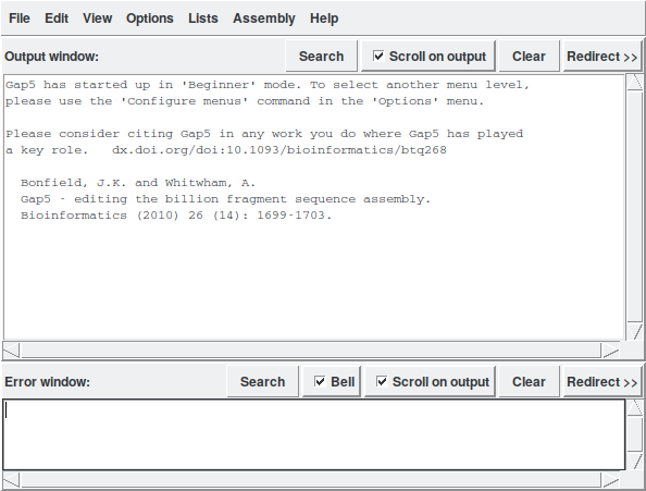
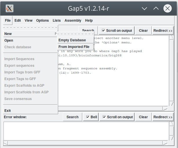
1. Data import
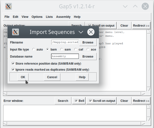
Open Gap5 and starting with the window in Figure 1. We can now import the BAM file by following the menu 'File - New - From Imported File' (Figure 2). This step opens another window (Figure 3) where we have to indicate:
- the input file (Filename: Mapping.sorted.bam), we can use the «Browse» button to search for it in our files;
- chose: bam;
- a name for our assembly: Assembly (for example);
- And then click 'OK'.
Gap5 starts working until we get our first representation of contigs in a new window called «Contig Selector» (Figure 4).
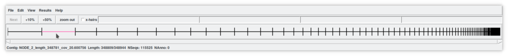
2. Contig Selector (Figure 4)
This representation reflects the order of the previously assembled contigs. If we move the mouse over the contigs, they are highlighted in pink and the name of the contig, its length, the number of sequences (reads) that compose it, and annotations, if any, are indicated below (Figure 4). This window also has the possibility of expanding forward (zoom + 10% and + 50%) or backwards (zoom out). We also find a checkbox «x-hairs selection» that activates a different pointer that will later show us its usefulness.
Selecting one or more contigs, highlights them in bold and they can be moved to another site by clicking with the mouse wheel on the site where they are going to. You can use the right mouse key to open other tools. Let's see a few of them. For a more detailed description you will have to wait for new posts on this blog. At the moment, it is better to see its main functions, and start understanding how it works.
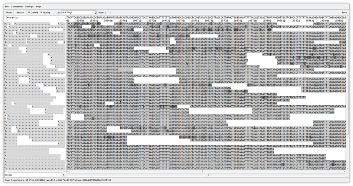
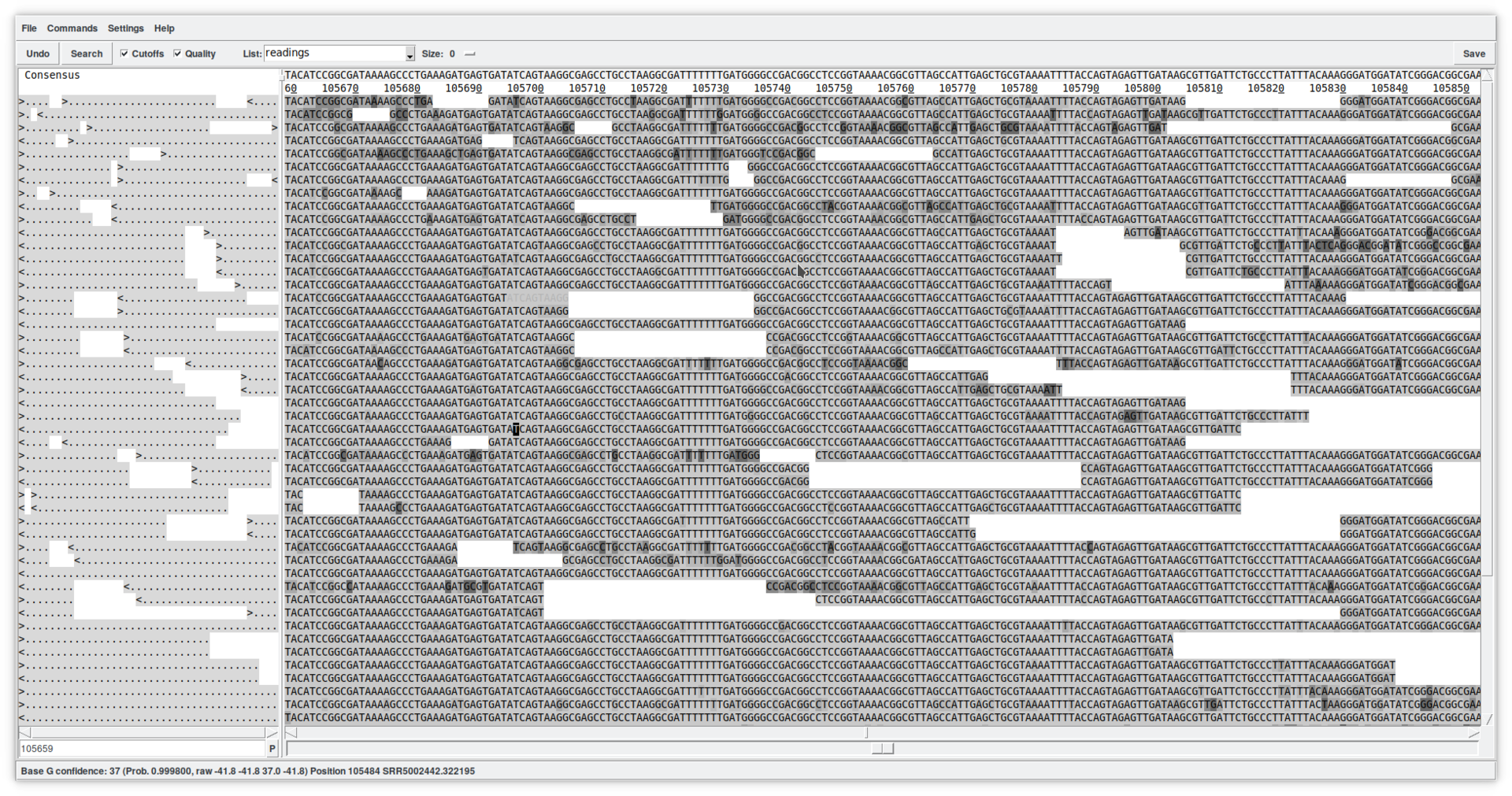
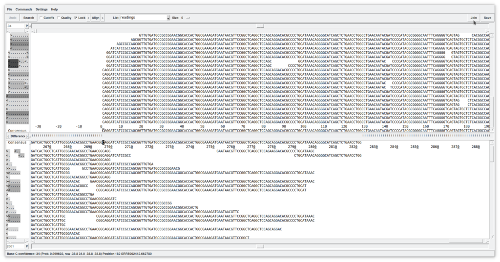
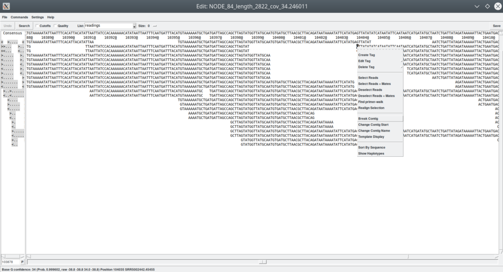
2.1. Edit contig (Figure 5)
This new window allows a detailed viewing of the contig's structure by showing the reads in the positions in which they have been mapped. This tool is quite complex and allows, among other things, to edit the sequences (simply by writing in the reads). You can view the quality of the reads by clicking on the «Quality» checkbox, as well as view any masked sequences by clicking on the «Cut-off» checkbox. At the top, the consensus is shown (which can be calculated using different algorithms). The direction of the reads is summarized on the left. In summary, this is just a first approach to the «Contig editor». It is a very powerful tool that, among many other functions, allows you to select reads for other uses, move them to other contigs, annotate them, or delete them from the database.
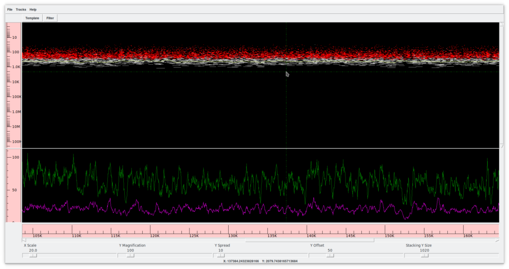
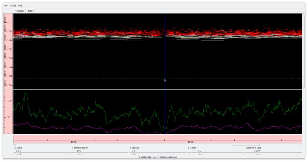
2.2. Template display (Figure 6)
This tool allows you to view a whole contig. At the bottom, there are several controllers that allow you to expand or collapse the contour frame in both dimensions. In the upper frame, the X axis shows the extension of the contig, while the Y axis shows the sequences (reads) in their position and extension relative to the contig. Colors provide information about the position, confidence, presence of forward and reverse mates in compatible directions, etc. The lower frame shows a graph summarizing the coverage and the quality of the assembly. A double click on any position opens the contig editor (previous point) at the corresponding spot.
2.3. Complement contig
The third tool that we can access by pressing the right mouse button on the contig, allows turning it into the complementary reverse direction.
3. Exploring the assembly
For this first approach I suggest we explore some of the main functions of the assembly edit menu. I apologize in advance for not explaining each item of the menu. I think it is more interesting at the moment to get excited with a global vision of the potential of Gap5, rather than to be discouraged by an overflow of information. To understand what we can do with Gap5 we start using the View menu.
- View - Contig selector. This command opens the window that we have already seen in point 2.
- View - Contig list. This command opens the list of contigs in a table format offering the same functions as the Contig selector.
- View - Results manager. Shows the history of applied commands.
- View - Find internal join. This command is probably one of the most important of all Gap5. It allows us to search for overlapping regions between contigs. Where the assembler has failed to close the contigs due to lack of information (possible, but the less likely option) or, more likely due to region resolution difficulty (due to repeated regions). Here is where the expert eye of the human researcher is needed to understand and solve the problem.
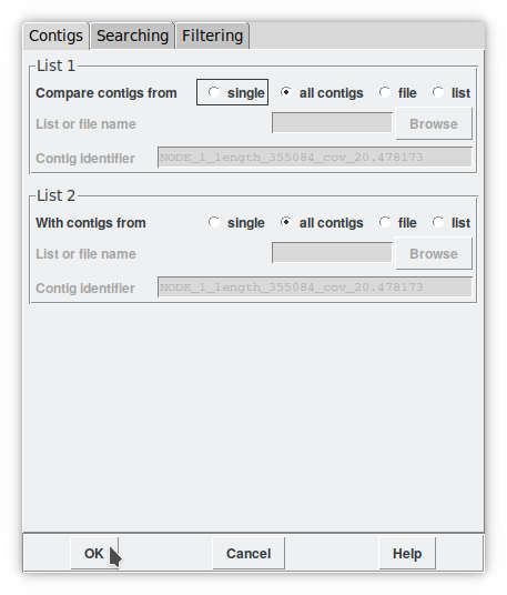
4. Find internal join.
By activating this command, a new window appears allowing us to set the alignment parameters set by default between the terminal regions of each contig (Figure 7). As a start, we can leave all the default parameters by executing an «all contigs vs all contigs». Then we can afford to be more specific, for example by focusing the process only on all contigs vs. a list or lists between two contig. The concept of «list» is another key point that allows us, for example, to create a list of dubious reads to disassemble and reassemble in a different context. By clicking on 'OK' the search starts. You may have noticed that the one-dimensional Contig selector transforms into a two-dimensional «Contig comparator».
Before continuing with the explanation of this tool, lets activate the checkbox «x-hairs» and, from the menu, «View - Diagonal display». What are we seeing (Figure 8)?
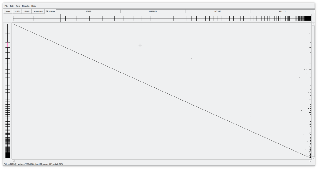
Now we have a two-dimensional assembly. All contigs in X against All contigs in Y. The crosshair indicates the possible point of union between a contig in X and another in Y. The contigs under our attention are shown in X and Y as coordinates where the cursor is pointing to. Try scrolling in both dimensions to see what happens.
Lastly, the four number boxes above indicate the cursor positions relative to the contig, and the cpmplete X-assembly and contig and complete Y-assembly respectively.
4.1. Joining contigs.
Another interesting features in this window are the black dots (in our assembly, mainly on the right side). These indicate regions of overlap between contigs (the «internal joins» that have been found). By zooming in we can visualize it more easily (Figure 9). Using the X and Y sliders we can quickly move through the assembly and, for example, find a line that represents a region of overlap between two contigs. By hovering over with the cursor the line turns pink and at the same time the two contig objects of the overlap are colored. Here is where the magic is done. By double clicking on the pink line, a window called «Join» opens with two up and down windows of the Contig editor more or less aligned. We can improve the alignment by clicking on the «Align» button that will execute another local alignment. Between the two contigs we can find some symbols «!» that tell us about mismatches. It is up to us to understand and decide whether these are errors or real variations in the genome.
Now the main question is: if these two regions are so similar, why hasn't the assembler joined them? My interpretations include:
- There are variations that make us suspect about repeated gene(s).
- There are too many errors.
- The total coverage at this point is so high that it makes us suspect again that they are perfectly identical repeated regions and that they probably can be allocated in two places in the genome.
- The coverage drops so much due to assembly errors thus, from a statistical point of view, it is not advisable to join them.
- The coverage drops due to sequencing difficulties (hard places to sequence, like those with too much methylation, etc.).
The assembly programs often overlook these possibilities (among others).
If you look at the end of the assembly (where all the smallest contigs remain), that's where possible junction points are accumulated and, incidentally, we can see how many contigs tend to join with a larger one and in the same place. This seems crazy and discouraging…
¡¡Welcome to the bowels of your assembly!!
Straightaway we can try to close a contig. In Figure 10 we can see a possible region of overlap between two contigs. After all my considerations and tests I decide that everything is correct, and I want to join them. At the top right there is a «Join» button that allows us to finish the job. Before allowing the union, another pop-up window appears, informing us about the overlap length and the percentage of errors. If we are satisfied, we can click Yes. The editor disappears and the two contigs are now merge into one. The most important point is that the contig still maintains all the reads and can rejoin others, as well as break if we detect any errors.
This nitpicking and scrutinous work can last for a few days (maybe even add some coffees, music, etc...) until we take advantage of all the useful information we have. This does not mean that we have to put all the contigs together into one, there is a lot of redundant information, but we do have to try to gather as much genetic information as possible.
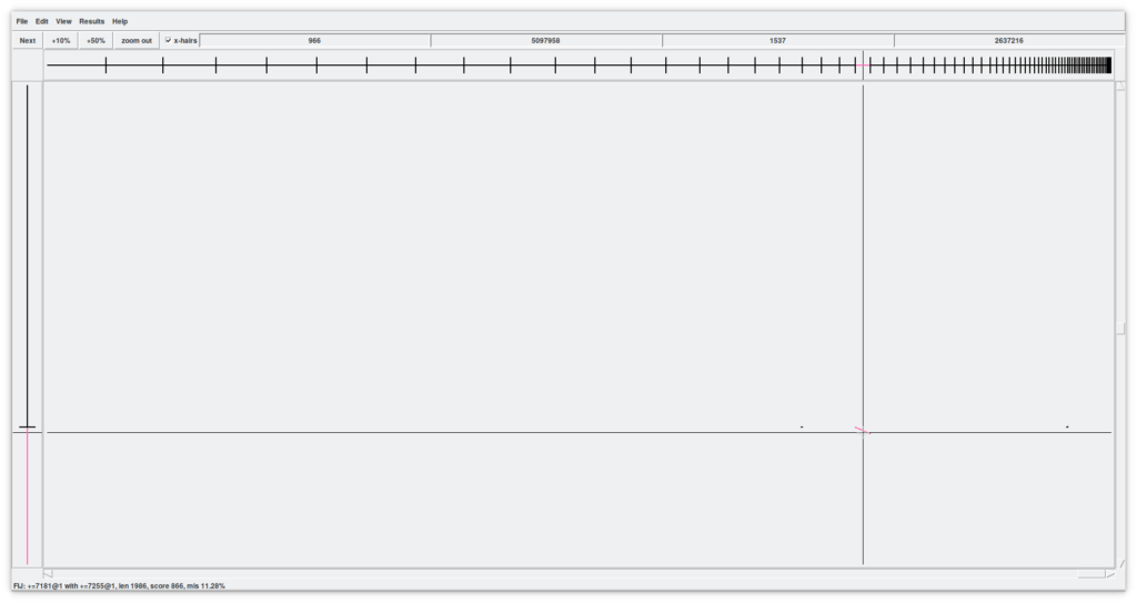
5. Breaking contigs (Figure 11 and 12)
If we find doubtful regions during our exploration, we can separate them. For example, using the «Template display», if we notice a site with a suspiciously low coverage. These are fairly frequent automatic assembly errors that I strongly suggest you check (Figure 11). A double click on the suspicious site opens the contig editor right in the same position (Figure 12). Indeed, I can see that very few readings support this union. I can decide to break the contig to try to join it with another that can give me better support. For this, I must move the cursor on the first base of the first reads of the new contig. Please, observe that this will not be a scissor hit. What we are separating are the reads without cutting them. This is very important to avoid making very serious mistakes. It must be recalled that the reads come from the real biology of the organism and, originally, they were real pieces of DNA that we cannot cut in the middle and rejoin with another piece. We would be generating artifacts. What is allowed, is to remove a read from one contig and paste it in another. In this case we would not be doing anything wrong (biologically speaking). Once the separation point has been identified (I have not used the term «cut point»), we click the right mouse button and select «Break Contig». It informs us about the positions of the separation and then we are left with the two contigs in two different windows.
I think the time has come to give you time to digest all this information. What we just went through in this entry is just the tip of the iceberg of the manual assembly review process. There are many more commands and options available to us, as well as many ways to deal with automatic assembly errors and repeated regions resolution.
Assembly errors are quite common, and it is true that the speed at which we are asked to work nowadays and the amount of data we can produce, especially in massive genome sequencing (where the adjective «massive» refers to the number of genomes) does not allow us to spend that much time playing with puzzles, but I think that there is beauty in each genome, and it is a real shame to ignore it or not give it our full attention, "simply" for being caught in the constant automation of processes, turning the researcher into part of the same automaton.
I say goodbye with the hope that you have found the time and the desire (if you liked it) to reach the end of this entry. For any doubt or question you can contact me at @gidauria.
Reference: The Staden Package. R Staden 1 , K F Beal, J K Bonfield. Methods Mol Biol. 2000;132:115-30. doi: 10.1385/1-59259-192-2:115. [PUBMEDID]. The web page: http://staden.sourceforge.net/.